

Getting things rolling, combining data in SAP Datawarehouse Cloud (1/2)!
We left you earlier this week with the promise that we would do a deep-dive into SAP Datawarehouse Cloud. And we did as promised!
You can read our previous blogs here
Our demo
At Interdobs we have a standard demo-set that we use for our own demo scenarios based on data coming from RDW. The RDW is the Netherlands Vehicle Authority in the mobility chain. RDW is the authority that gives out license plates, but is also responsible for the yearly MOT inspection and keeps track of all data of the cars driving around in Holland. The nice thing is that RDW stores data about all their processes and makes this available via the Open Data protocol.
Basically we have two datasets in this scenario: the problems that have been recorded by the garage and was send towards RDW and the recalls coming from the dealers. In our demo we want to combine the two datasets to get information about our favourite car: Peugeot 308.
Getting data in
We had two main data sources for our data: a flat-file and data from our HANA database. The challenge here was that the flat-file upload is limited to 20mb, and our file containing all the recalls is about 160 mb. Luckily it is possible to keep uploading flat-files into the same table, which are automatically appended to the previous loads.
Uploading is a piece-of-cake: SAP Datawarehouse Cloud almost instantly recognizes what is in the file and is able to split the columns. I can remember doing this same exercise with the file import from HANA Studio and that took me quite a bit longer because the file needed to be really clean before I could import it into HANA.
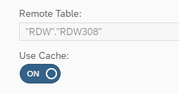
The second dataset is the data with the recalls coming from the dealers. We have this data in a table in our HANA system and via a remote source (running via SDI in this case) we connected it to DWC. SAP recommends at this stage to use replication for remote sources to get the best performance out of the data. Replication is done very easily by using the “Cache” slider under the table options.
About the different adapters
While I am on the subject of connections: we currently have two adapters available to connect with our SAP HANA / SAP BW system. The first adapter is the one mentioned above and re-uses the technique of Smart Data Integration, the second adapter is the ABAP adapter. The ABAP adapter makes SAP BW objects available for SAP Datawarehouse Cloud, but with different technical names than you might expect (probably something that will be changed/fixed down the line). Obviously we tested both the HANA and the ABAP adapter and although the HANA adapter seems a bit faster, the ABAP adapter surprised us in speed and the functionality to show our HCPR from SAP BW within a few seconds! You can get more information on connections in the following YouTube clip.
Using a beta
While using this product you sometimes forget that you are working with a beta product, only the “unavailable” icons in the left bar remind you. That is until you return after a quick break and buttons on the screen are in different (and smarter) places all of the sudden! This only shows how committed SAP is and the amount of work that is being put into this product.
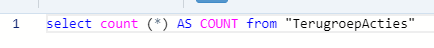
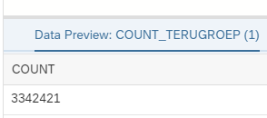
“Unavailable” functions also mean that sometimes you miss something that you really want to use. For example you want to show the audience of your blog that the dataset used in your demo is quite extensive, to prove that we are not lying about the performance. At this time we don’t have the availability to show the amount of records in a table with standard functionality. This is easily overcome by using a a SQL view with a simple count.
Back to the data-model
Via the Data Builder we created our Graphical View that contained our demo data:
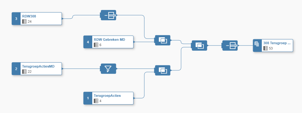
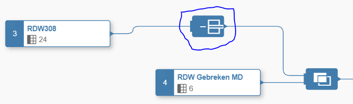
Since I already briefly went over the data builder last time, let’s take some more time to go over the individual components. In below screenshot you can see that we are joining the RDW dataset with the faulty data of the Peugeot 308 to some master-data containing a translation from the error code to something that we really understand. The object in the blue circle is there to remove some columns from the source table before joining it to its master-data.
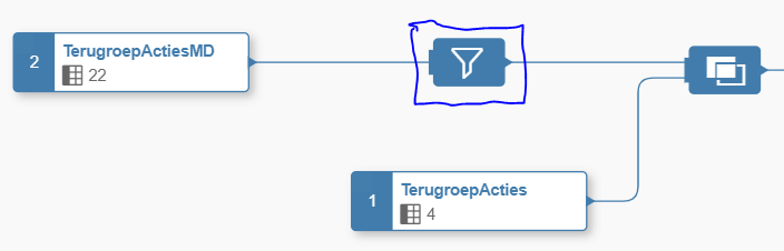
On the other side you clearly see the filter icon, which we use to filter out only the recalls coming from the Dutch Peugeot importer.
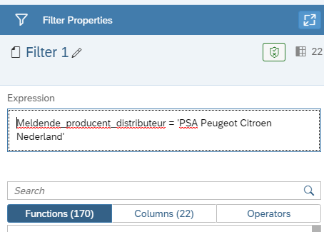
As you can see in the image below we wrote a very straight on expression to filter our data, but look at the 170(!) functions that are already available to do some kind of filtering on your dataset.
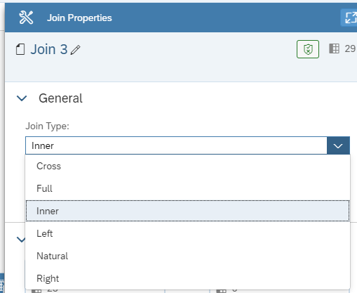
Joining the dataset is done by drag-and-dropping the elements that you want to join. Currently we have already all the possible joins you need in the toolbox available:
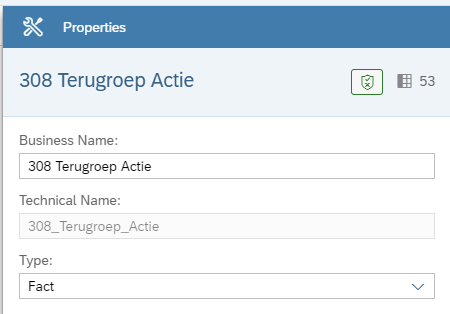
Lastly we have the “result” node, which is comparable with the last node in a HANA view. Just create your view and in the final step determine what type of view you created. One important thing here is that when you want to show your data in the data visualizer (SAC embedded in Data Warehouse Cloud) as type “Fact”.
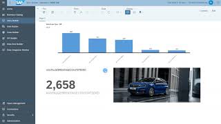
Data visualizer
This is where Martijn van Foeken will take over in a few days! He will take you through all the capabilities of the data visualizer in SAP Datawarehouse Cloud. And for me this will be extra exciting because I can finally find out the quality of my 308!
Want to see SAP Datawarehouse Cloud for yourself? Please watch the movie recorded by Ronald Konijnenburg below. If you want to know more about SAP Datawarehouse Cloud after reading this blog and seeing the movie, please don’t hesitate to contact us!